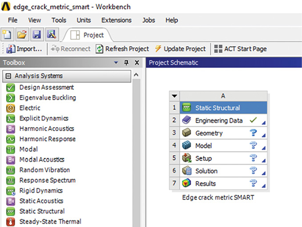
In this new article, Tony Abbey revisits ANSYS Workbench to carry out a series of Fracture Mechanics analyses. Fig. 1 shows a New Static Structural analysis in the Project Window. Images courtesy of Tony Abbey.
Latest in Finite Element Analysis FEA
Finite Element Analysis FEA Resources

Latest News
May 1, 2019
I am revisiting ANSYS Workbench to carry out a series of Fracture Mechanics analyses (see DE February 2019 article). I was particularly interested in the new ANSYS Separating Morphing Adaptive Re-meshing Technology (SMART). The acronym is a bit of a mouthful, but is an accurate description of the solver’s capabilities. As the crack front moves forward, the mesh splits around it, and the surrounding zone is remeshed.
Fig. 1 shows the project opened and saved. A Static Structural analysis is dragged to the Project Schematic window and named as “Edge crack metric SMART.”
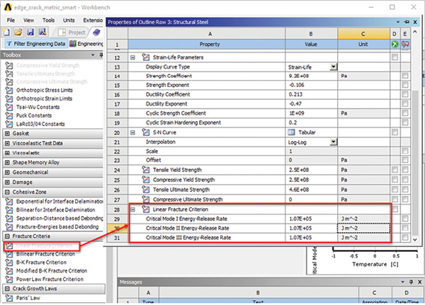
The Engineering Data tab allows access to the material definition. I have accepted the default material, which is a generic Steel. I will start with a static analysis—an overload that creates a nonlinear fracture surface (i.e., a crack) in the model. The key material property is the Fracture Toughness, which is defined in a Fracture object, as we will see shortly.

The test model is an edge crack in a thick plate. The geometry was created externally and imported into SpaceClaim. The layout is shown in Fig. 2.
With the geometry in place, double-clicking on the Model tab in Fig. 1 launches ANSYS Mechanical. There are several tasks to perform here specific to the fracture mechanics analysis.
The SMART fatigue option requires a tetrahedral element mesh. The mesh size needs to be refined around the crack tip. I have used a sphere of influence method based around the geometric edge running through thickness.
I must select three named geometric regions to define the crack. These are the crack edge, the top surface of the crack and the bottom surface of the crack. Each of these regions is then associated with a node set for use in the analysis.
A local coordinate system is defined for the crack tip. The components indicate crack propagation direction (x) and crack opening direction (y).
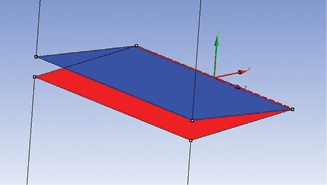
FIG. 3: Named surface, edge and coordinate system for crack.
The selected entities and coordinate system are shown in Fig. 3.
From the Command ribbon, the option for Fracture is chosen. Further options for introducing a crack are: Arbitrary Crack; Semi-Elliptical Crack and Pre-Meshed Crack.
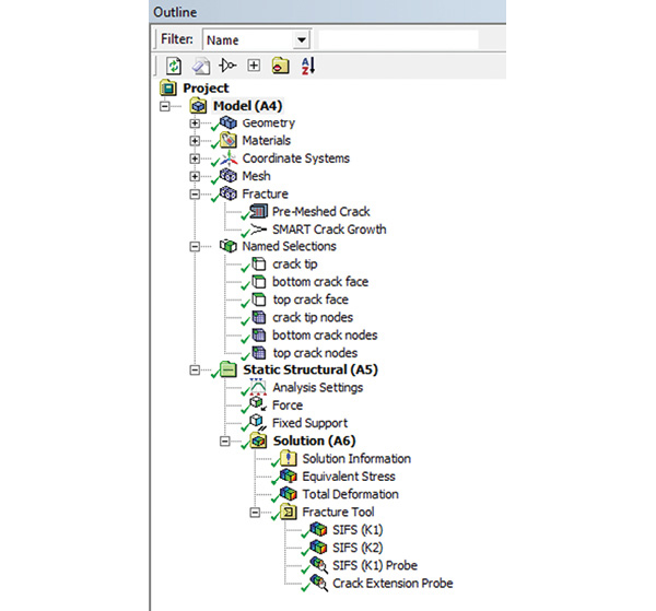
The Pre-Meshed Crack option is selected. Fig. 4 shows the complete set of objects used to set up the Static Fracture analysis.
Within the Pre-Mesh Crack object, the Node sets created previously are allocated to the crack front, and the crack top and bottom faces. The crack coordinate system is referenced. The number of solution contours is set to 5. These are the “loops” through the mesh around the crack tip, which are used to evaluate the Stress Intensity Factor by integrating the crack tip region strain energy. The Fracture Mechanics approach avoids the stress singularities at the crack tip in the analysis.
In the Fatigue menu ribbon, three methods are available to model the crack front and its growth: Interface Delamination, Contact Debonding and SMART Crack Growth.
SMART Crack Growth is selected, and the menu is shown in Fig. 5.
The Pre-Meshed crack object is selected, the option to carry out a Static Fatigue analysis is chosen and the Critical Fracture Toughness is defined. The Stress Intensity Factor method is selected in this case. The crack will propagate when the calculated Stress Intensity Factor, K exceeds the Fracture Toughness Kc. This calculation is done along the distributed crack front, and the distribution of Stress Intensity Factor will control the adapting crack front shape. The Failure Criteria can also be set to the J-Integral method.
Fig. 4 shows output requests and includes general stress and displacement contours as well as fatigue-specific probes. The main fracture mechanism in this model is the crack tensile opening Mode 1, which calculates KI. The probe SIFS (K1) reports these values.
I have also included a probe for the in-plane shearing Mode 2, which calculates KII as SIFS (K2). These values are secondary for this configuration but may become important for a crack that changes direction significantly with a resulting shear stress environment. I have also included a crack extension probe to monitor the crack growth. Each of these probes will produce an XY plot.
I have constrained the bottom surface of the test piece and applied a vertical force of 1.5E5N. The initial crack length is 6.4 mm. A manual calculation gives a value for KI of 6.152E7  . This is below the Critical Kc of 1.5e8 input in Fig. 5. The component will not fracture under this loading. The main objective is to check the value and distribution of KI.
A Static Fracture Analysis
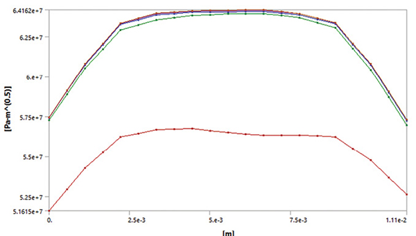
After launching the analysis, the distribution of KI along the crack front is shown in Fig. 6.
The manual calculation referenced is for an assumed infinitely deep plane strain section and is a one-dimensional (1D) approximation. The value matches the finite element analysis (FEA) distribution well. The edge effect can be seen in the 3D model.
There are five curves shown in Fig. 6. These represent the five contours requested in the Pre-Mesh Crack object. They are used to check for convergence of the KI value. The first curve is from a contour close to the crack tip; the other curves represent contours at increasing distances. The curves converge quickly, showing the mesh is adequate.
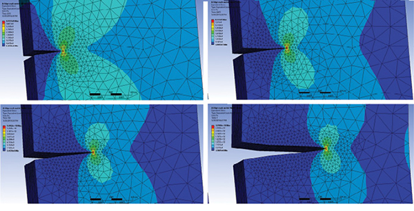
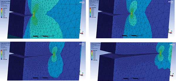
I then increased the load to 7E5N, which gives a KI of 3E8 for the initial crack length of 6.4 mm. This is greater than Kc and results in a static fracture. Running the model with 40 Substeps results in a crack extension of 14.5 mm. The crack extends to just over 50% of the plate width. Fig. 7 shows the changing crack and mesh configuration. The maximum stress contours are adjusted at each step.
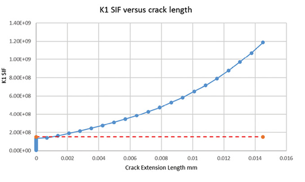
Fig. 8 shows the average KI as the crack progresses, together with the threshold Kc, shown as an orange dashed line. The location to sample along the crack front can be selected, and I have used the midpoint of the crack front.
No geometric nonlinearity allowed—so the crack length here is limited realistically unless we use a displacement control. The eccentricity created by the crack would result in very large bending stresses in the residual material, as the crack runs out, with a resulting complex failure mechanism. A crack extension limit can be defined to prevent an unrealistically long crack.
A Fatigue Fracture Analysis
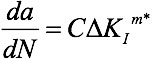
The fracture type in the SMART Crack Growth object is now set to Fatigue—an investigation of the Fracture Mechanics response under a cycling load. This requires additional material data definitions for the Paris Law. The Paris Law is defined by:
where:
 is the rate of crack growth per cycle;
 is the Stress Intensity Factor range (based on maximum stress and minimum stress);
C is the Paris Law coefficient; and
m* is the Paris Law exponent.
The additional data required are the coefficient and exponent. The units of the coefficient material data are tricky as they embody the exponent m in the conversion. (I will be writing about non-intuitive units in a future article!)
The material data I used was:
C = 1.9e-29 : units are m/(MN m^-3/2)^m*
m* = 2.8 : dimensionless
The Stress Ratio is used to define the ratio of minimum stress to maximum stress. This gives the stress range and hence the Stress Intensity factor range. In my case, the stress is cycling from zero to maximum, so the ratio is 0.0. If the stress was fully reversed, the ratio would be -1.0.
The load is dropped to a much lower level of 27.0 KN, appropriate for a continuous cyclic operational loading.
A data probe is added to report the number of cycles for each crack increment.
A solution for an approximate 1D solution can be found using this expression:
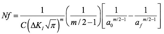
ao is the initial crack length and
af is the final crack length.
The catch is that the Stress Intensity Factor range, is a function of crack length, so the equation has to be evaluated numerically. I have an Excel spreadsheet to perform this 1D approximation.
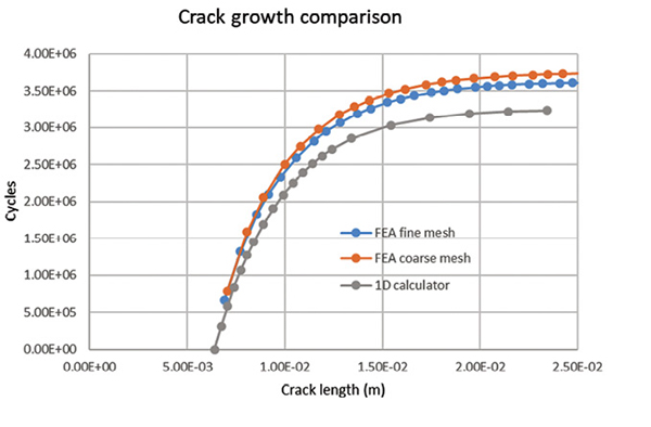
After I run the fatigue analysis, the probes are used to recover the Number of Cycles vs. Crack Length, as in Fig. 9.
Two ANSYS runs are carried out: a relatively coarse mesh and a finer mesh. The local element size is reduced from 0.8 mm to 0.65 mm. There is clear evidence of convergence with the life to create a 25 mm crack reducing from 3.74 E6 cycles to 3.62 E6 cycles. The 1D model provides a useful comparison with a life to 25 mm of 3.24 E6 cycles.
The convergence accuracy is based on both mesh size and initial crack step length. Both are controlled in ANSYS by the mesh size. So, finding a sufficiently fine mesh is important.
The crack extension through life is shown in Fig. 10. The stress contours are adjusted to maximum values at each step.
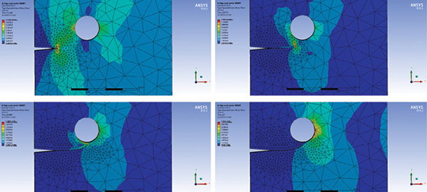
A hole is now inserted in the SpaceClaim model. The project is updated and automatically remeshed. No other modification is required, and the analysis is relaunched. The result of the modification is shown in Fig. 11.
The crack is now attracted to the hole and joins it on the far side from the crack origin. The crack is then arrested and there is no further extension. The crack is arrested at around 8.631 E5 cycles and the structure is damage tolerant with respect to this particular initial crack and loading.
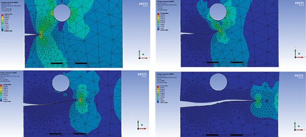
The SpaceClaim geometry is modified by dragging the hole further away from the crack axis. The model is updated and again automatically remeshed. The results of this analysis are shown in Fig. 12.
The crack is influenced by the hole but bypasses it. Interestingly, the crack growth rate speeds up compared to a plate without a hole. The number of cycles to reach the critical crack length has dropped to 1.09 E6 cycles. This is around one-third of the total for the plate without a hole. The relationship between the hole and the crack is clearly important. The hole can arrest the crack—or speed it up!
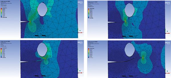
A more arbitrary shaped hole was investigated, positioned at the same point, but elongated slightly in the vertical axis. The results of this analysis are shown in Fig. 13.
The hole attracts the crack but is not a strong enough influence to arrest it. It also acts to speed up the crack propagation further with 1.2 E5 cycles to the critical length.
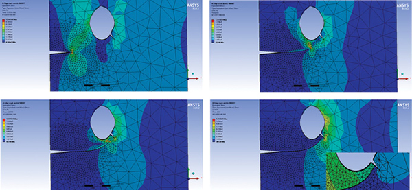
Finally, a sharp notch in the hole edge was modeled to see if the crack would be attracted. This is shown in Fig. 14.
The sharp notch does attract and arrest the crack. It now takes 6.76 E5 cycles to reach this point. The notch is intercepted partway along its length. This is shown more clearly in the displacement plot, which is inset in the last frame of Fig. 13. Experimenting with the notch shows there is a critical length to attract the crack to an arrested state. Below that length the notch acts to accelerate the crack.
The workflow to set up the crack and define the fracture parameters is straightforward. The direct interface with SpaceClaim geometry allows for rapid “what-if” studies. This is a versatile tool and I have only shown one crack type.
The Arbitrary Crack and Semi-Elliptical Crack look useful in creating cracks in more complex geometry. The other fracture solution methods, Interface Delamination and Contact Debonding, provide solutions for pre-defined crack paths, such as along bond lines.
More Ansys Coverage
Subscribe to our FREE magazine, FREE email newsletters or both!
Latest News
About the Author
Tony Abbey is a consultant analyst with his own company, FETraining. He also works as training manager for NAFEMS, responsible for developing and implementing training classes, including e-learning classes. Send e-mail about this article to DE-Editors@digitaleng.news.
Follow DE